

Reading fewer tokens does not necessarily make a language model fast. The system may still spend most of its time deciding which tokens to read. Latent Sparse Attention (LSA) addresses this search cost by grouping keys in a learned space and guiding queries through representatives of those groups.
D-LSA adapts an existing model through indexer distillation; N-LSA learns with the model from the outset. This analysis separates their mechanisms, measured results and remaining limitations, using the version of the paper examined in the source article.
The paper and the version examined
The paper is Latent Sparse Attention: Towards Subquadratic Ultra-Long Context Attention, by Ales Kubicek, Andrea Caciolai, Liangzu Peng, Sukrit Sumant, Benjamin Hoover, Fraser Greenlee, Ruairidh M. Battleday, Radim Urban, Torsten Hoefler and James C. R. Whittington. Urban and Hoefler are affiliated with ETH Zurich; the other listed authors are affiliated with Prefrontal AI.
The analysis concerns arXiv:2610.42147v1, submitted on 30 October 2026, with DOI 10.48550/arXiv.2610.42147 and a CC BY 4.0 licence. It is a preprint, not presented here as a peer-reviewed publication. The original Figures 3–7 and Table 3 are retained. Measurements reported by the authors are distinguished from the technical interpretation offered here.
Why sparse attention can still be expensive
A query represents the information currently sought, a key provides a basis for comparison, and a value supplies the representation actually read. Full attention compares each query with preceding keys, so prefill work generally grows quadratically with context length T. Sparse attention first selects a subset, but its indexer can still scan all keys or contiguous blocks.
In the paper’s Figure 2 experiment, indexing accounted for 98% of sparse-attention prefill time at 10 million tokens. That result concerns one GLM-5.3-Flash global attention layer on one H200, measuring the final 32,768-query chunk. LSA groups keys by similarity in a learned vector space; “semantic” clustering does not mean that a person assigns topic labels.
Clusters locate tokens; the original keys and values supply attention
In the principal D-LSA configuration, keys are projected into a 64-dimensional index space and normalised. Four consecutive keys are pooled, and similar keys are merged within 512-token cluster blocks. Ward’s criterion favours merges with the smallest increase in within-cluster dispersion. Buckets average eight keys, with a maximum of sixteen; completed blocks are not subsequently reclustered.
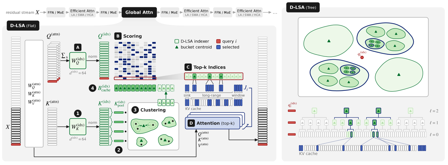
Each bucket stores its centroid and a map back to original key positions. A query scores centroids, selects promising buckets and expands their position maps into the original indices, within a long-range token budget. Sink tokens at the beginning and a recent-token window are also included. The window covers the newest block before it is clustered. Centroids support retrieval; they do not replace the original keys and values in the final attention computation.
Flat search scores every bucket centroid. With fixed bucket size, work per query remains linear in T and prefill indexing remains asymptotically quadratic. Tree search adds higher-level groups and beam search. With a fixed candidate budget at each level, the number of scored centroids per query is O(log T), giving O(T log T) prefill indexing. The subquadratic complexity claim belongs specifically to this Tree design.
D-LSA learns where an existing model looks
D-LSA freezes the pretrained model and learns small layer-specific query and key projection matrices and a training temperature. The original attention distribution supplies the teacher signal. Distillation scores all keys directly and does not include clustering in the loss calculation.
The authors report 352 million training tokens drawn from documents of 16k to 1M tokens. They did not then retrain the whole model under sparse attention because of the cost. The evaluated models start from different baselines: full attention in Qwen-3.8-27B and existing sparse attention in GLM-5.3-Flash. A separate Training-Free variant uses principal directions without distillation; it should not be confused with the principal D-LSA results.
N-LSA learns directly from next-token prediction
N-LSA uses no teacher model. It clusters the attention keys themselves and scores a bucket using the maximum similarity between its centroid and the query heads, without adding dedicated index projections. The selection operation stops gradients; learning proceeds through attention to the selected keys, sink and recent window. The implementation uses no auxiliary loss or additional parameters.
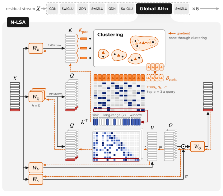
The experiment used a roughly 0.5-billion-parameter, 24-layer hybrid model. Every fourth layer was attention and the rest were Gated DeltaNet layers. Training comprised 4k-context pretraining and a 128k-context learning-rate decay phase. Only Flat search was evaluated for N-LSA, so this does not establish native Tree training at large-model scale.
Evaluation tasks and context extension
D-LSA was evaluated on MMLU-Pro, GPQA-Diamond, AIME25, MATH500, LongBench v2 and RULER. Some benchmarks used subsets because ultra-long-context evaluation is expensive. RULER used 100 prompts per task through 1M tokens and 20 beyond that length.
The new PaperTrail benchmark inserts constructed factual clues into scientific papers and tests retrieval from one paper, links between two, and chains involving three or more. It does not directly measure scientific discovery in real research. Contexts extended to 10M tokens. Qwen-3.8-27B used YaRN context extension, while GLM-5.3-Flash has no explicit positional encoding requiring the same treatment. These tests are not confined to each model’s original advertised context range.
Accuracy depends on the model, length and search design
For Qwen-3.8-27B, D-LSA Flat remained within five points of full attention through 1M tokens. At 10M, RULER was 63.9 versus 59.9 and PaperTrail 29.1 versus 19.8 in favour of Flat. Those are observations under the reported tasks and settings, not a general rule that reading fewer tokens improves accuracy.
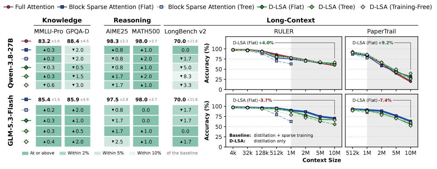
For GLM-5.3-Flash, Flat stayed within three points of its sparse baseline through 1M, but trailed by up to eight points between 2M and 5M. At 10M the RULER gap was within four points. Tree scored 55.8 there against Flat’s 66.8. Both models also faced harder tasks as context grew. Matching an increasingly weak baseline and solving the task well are different achievements.
Layer speedups and whole-model serving latency
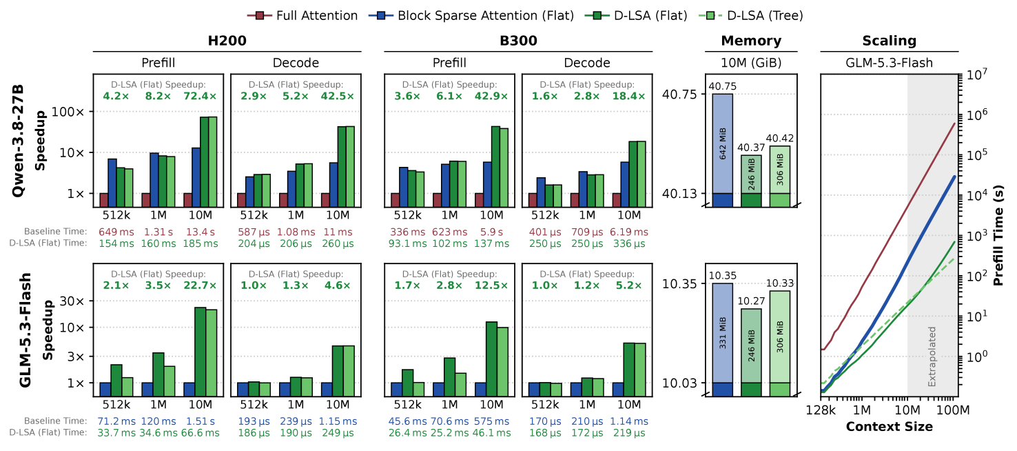
On one H200 at 10M tokens, a D-LSA attention layer achieved prefill/decode speedups of 22.7×/4.6× over GLM-5.3-Flash’s sparse attention and 72.4×/42.5× over Qwen-3.8-27B’s full attention. Prefill measured the last 32,768-query chunk; decode measured one step for one request. These are not end-to-end request speedups.
Under SGLang, Qwen-3.8-27B D-LSA Flat on H200 at 10M improved time to first token (TTFT) by 9.21× and time per output token (TPOT) by 2.87×, using TP8 and DCP8. Table 3 gives baseline times in the first row of each block and relative speedups in the remaining rows, so the hardware and parallelism matter.
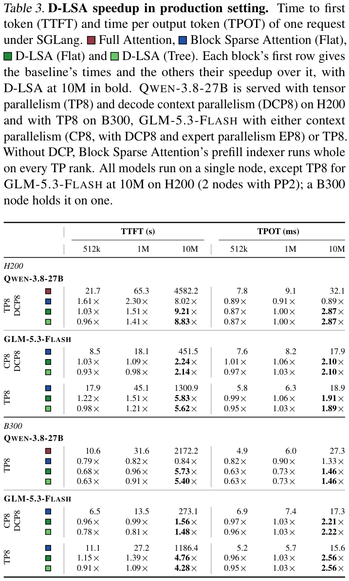
For GLM-5.3-Flash on H200, the CP8 setup gave TTFT/TPOT improvements of 2.24×/2.10×; TP8 gave 5.83×/1.91×. The specified 10M H200 TP8 configuration used two nodes with PP2. Shorter contexts can be slower: Qwen-3.8-27B Flat on B300 at 512k reported 0.68× TTFT and 0.63× TPOT. A value below one indicates a slowdown because selection and clustering overhead can exceed the attention work saved.
Native training trades speed against memory
At 128k tokens, N-LSA’s forward and backward passes through one attention layer were 1.6× faster than full attention. The whole hybrid model’s decay phase was 1.24× faster at the same validation loss, 1.085 for both methods. Layer and whole-model gains differ because only every fourth layer uses attention.
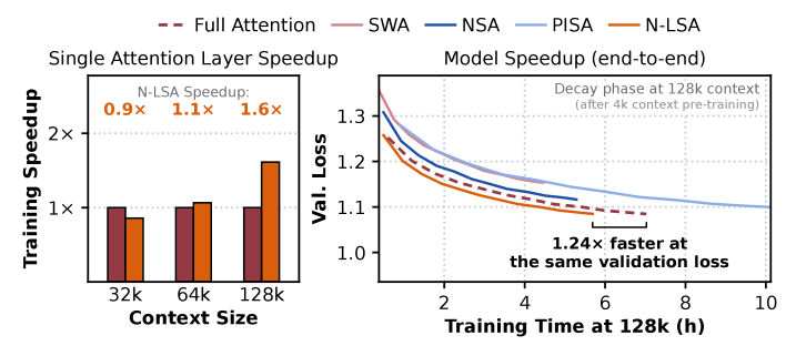
Peak memory was higher: 6.8 GiB per layer for N-LSA against 5.8 GiB for full attention. Keeping selected indices for the backward pass contributes to that cost. Training speed alone therefore does not establish a memory saving.
Limits of the evidence
LSA reduces the cost of finding keys, not the amount of original KV data that must be stored. The KV cache still grows linearly with context. Figure 6 extrapolates beyond 10M tokens; the large projected gains at 100M are not measured results. In the reported single-request decode experiments, D-LSA Tree also used Flat search, so the decode gains cannot all be attributed to tree traversal.
Native training evidence is limited to the roughly 0.5B model, 128k context and Flat search. Larger models, longer contexts and native Tree training remain open questions. Benchmark subsampling and context extension also limit direct comparison with an actual service’s request concurrency, latency targets and document distribution.
Assessing LSA’s technical contribution for patent work
The technical problem is the selection bottleneck that remains even after sparse attention reduces what is read. The meaningful combination is the learned retrieval space, clustering within bounded blocks, centroids and original-position maps, query-dependent bucket selection, and a return to the original keys and values. Sink and window handling complete that processing chain; Tree adds a hierarchy of candidate reduction.
The distinction from contiguous-block summaries lies in which keys are grouped, while the distinction from scanning all groups lies in the search path. Distilled and native implementations connect this structure to learning in different ways. A useful technical assessment relates those configurations to the measured gains and costs: ultra-long-context speed, accuracy loss with Tree, short-context overhead and increased N-LSA memory. A speedup figure alone does not describe the contribution.
The original figure labels and forms are preserved; the text explains the source material.
Paper reviewed: Latent Sparse Attention v1
Discuss the technical structure and patent implications of AI systems with IPLEX.
Explore our AI and patent practice